This Quickstart will demonstrate how to run model predictions inside Snowflake using the orbital R package and the Snowflake Native Posit Workbench App.
With the orbital package, you can:
- Speed up model predictions by running them directly in a database like Snowflake.
- Easily share your models with others by storing predictions in a Snowflake table or view.
We'll use loan data from LendingClub to build an example model in this Quickstart.
What You Will Build
- An RStudio Pro IDE environment to use within Snowflake.
- An R Script that builds a model workflow using the tidymodels framework, then transforms that workflow into Snowflake SQL with orbital.
- A table or view of model predictions, ready to share with others.
You can follow along with this Quickstart guide, or look at the materials provided in the accompanying repository: https://github.com/posit-dev/snowflake-posit-quickstart-orbital.
What You Will Learn
- How to create a tidymodels workflow that bundles pre-processing and modeling steps.
- How to transform that workflow into Snowflake SQL with orbital.
- How to run model predictions on Snowflake using orbital.
- How to create Snowflake views to store and share model predictions.
Pre-requisites
- Familiarity with R
- Familiarity with modeling in R with the tidymodels framework
- The ability to launch Posit Workbench from Snowflake Native Applications. This can be provided by an administrator with the
accountadminrole. - A Snowflake account with an
accountadminrole or role that allows you to:- Create databases, schemas and tables
- Create stages
- Load data from S3
- Access to Posit Connect
Before we begin there are a few components we need to prepare. We need to:
- Add the Lending Club data to Snowflake
- Launch the Posit Workbench Native App
- Create an RStudio Pro IDE session
- Install necessary R Packages
Add the Lending Club Data to Snowflake
For this analysis, we'll use loan data from LendingClub. We've made the data available in an S3 bucket.
The data contains information for about 2.3 million loans from the Southern US states.
Add Data
In Snowsight, click Create > SQL Worksheet. Copy this SQL code and paste it into the worksheet. Run the code to create the database and table you'll need for this Quickstart.
You may need to change the role granted usage from SYSADMIN to your desired role.
Confirm Data
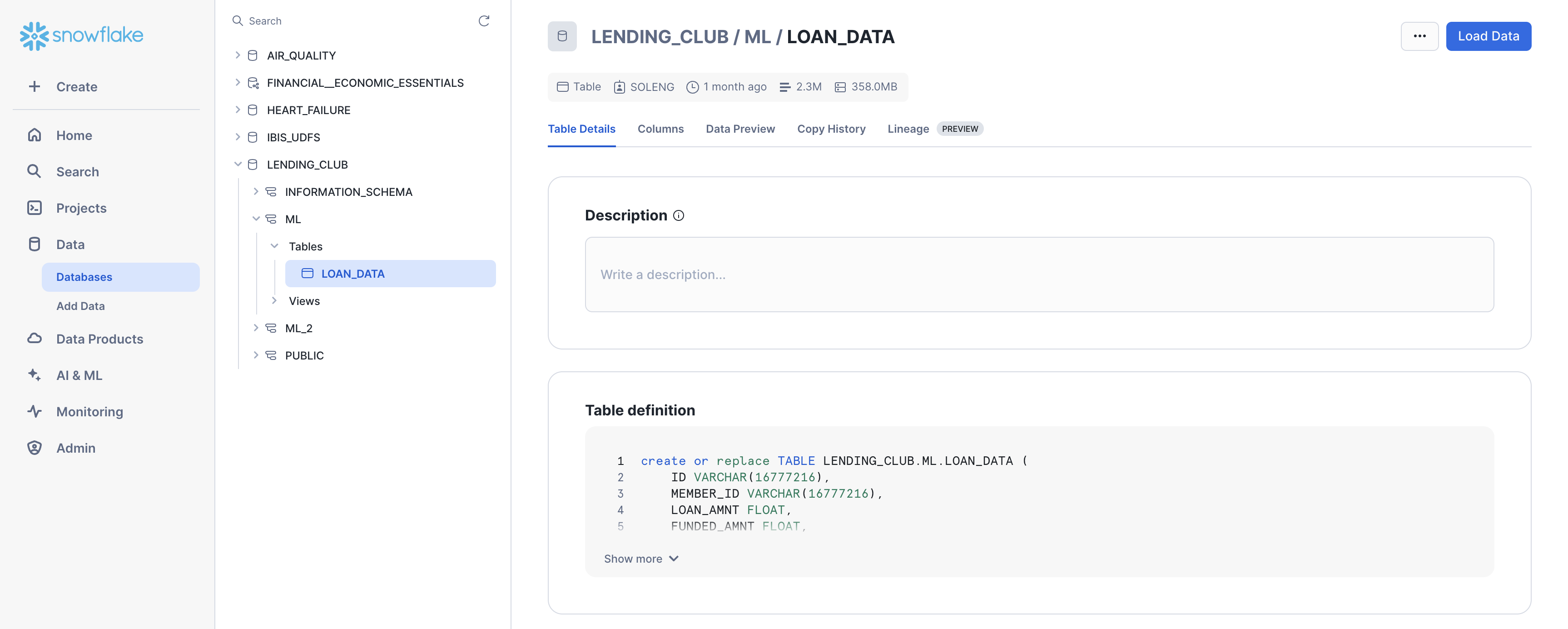
After running the code, you should be able to see the Lending Club data in Snowsight.
Navigate to Data > Databases and select the database where you added the data (e.g., LENDING_CLUB). Expand the database, schema, and tables until you see the LOAN_DATA table.
Launch Posit Workbench
We can now start the modeling process with the data using the Posit Workbench Native App. The Posit Workbench Native App allows users to develop in their preferred IDE in Posit Workbench with their Snowflake data, all while adhering to Snowflake's security and governance protocols.
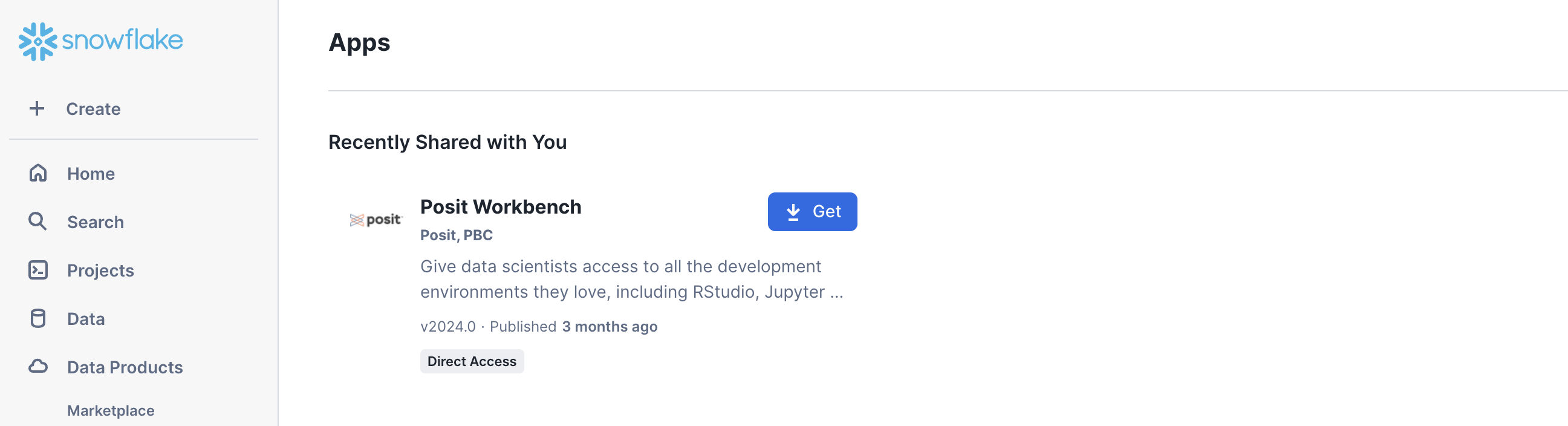
Step 1: Navigate to Apps
In your Snowflake account, go to Data Products > Apps to open the Native Apps collection. If Posit Workbench is not already installed, click Get. Please note that the Native App must be installed and configured by an administrator. Installation and configuration also require a valid license file from Posit.
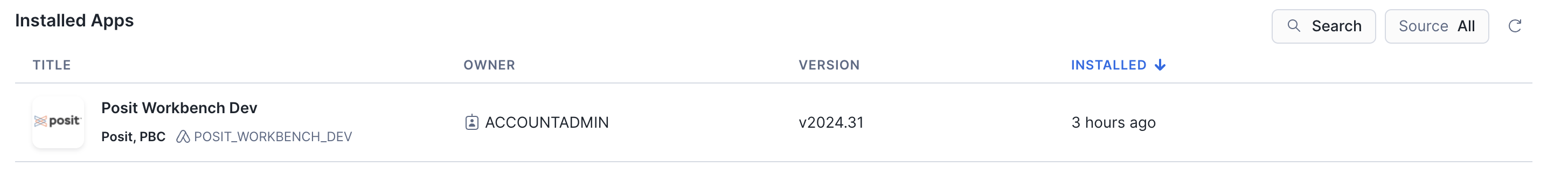
Step 2: Open the Posit Workbench Native App
Once Posit Workbench is installed, click on the app under Installed Apps. If you do not see the Posit Workbench app listed, ask your Snowflake account administrator for access to the app.
After clicking on the app, you will see a page with configuration instructions and a blue Launch app button.
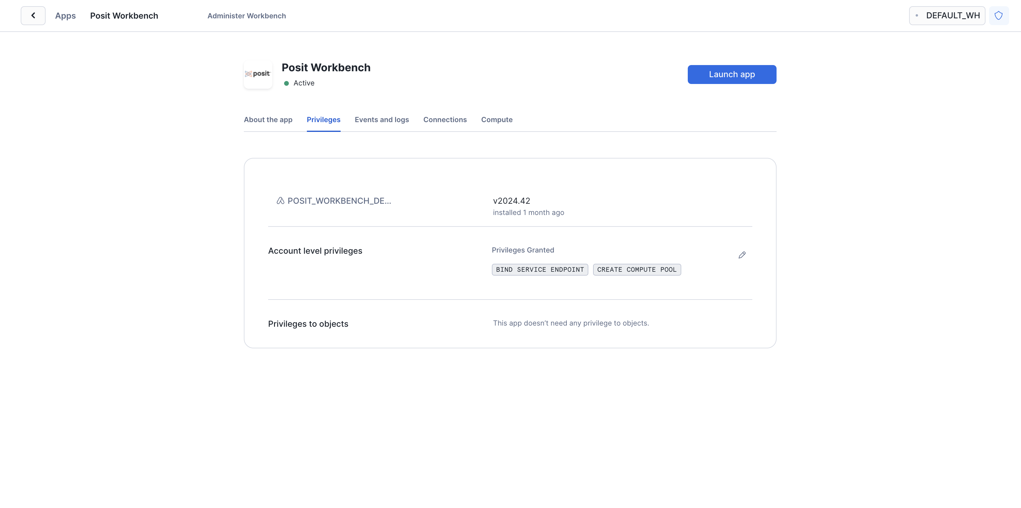
Click on Launch app to launch the app. You may be prompted to first login to Snowflake using your regular credentials or authentication method.
Create an RStudio Pro Session
Posit Workbench provides several IDEs, such as RStudio Pro, JupyterLab, and VS Code. For this Quickstart, we will use RStudio Pro.
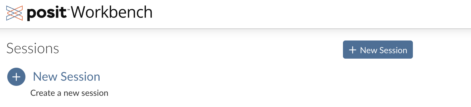
Step 1: New Session
Within Posit Workbench, click New Session to launch a new session.
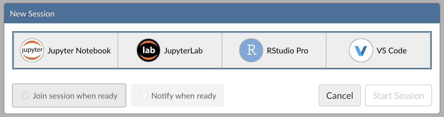
Step 2: Select an IDE
When prompted, select RStudio Pro.
Step 3: Log into your Snowflake account
Next, connect to your Snowflake account from within Posit Workbench. Under Session Credentials, click the button with the Snowflake icon to sign in to Snowflake. Follow the sign in prompts.
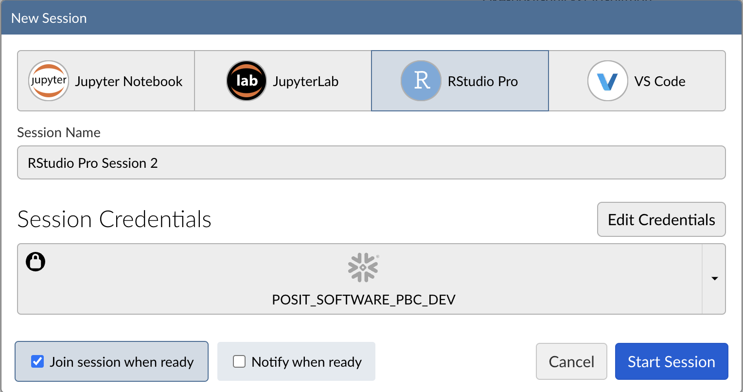
When you're successfully signed in to Snowflake, the Snowflake button will turn blue and there will be a check mark in the upper-left corner.

Step 4: Launch the RStudio Pro IDE
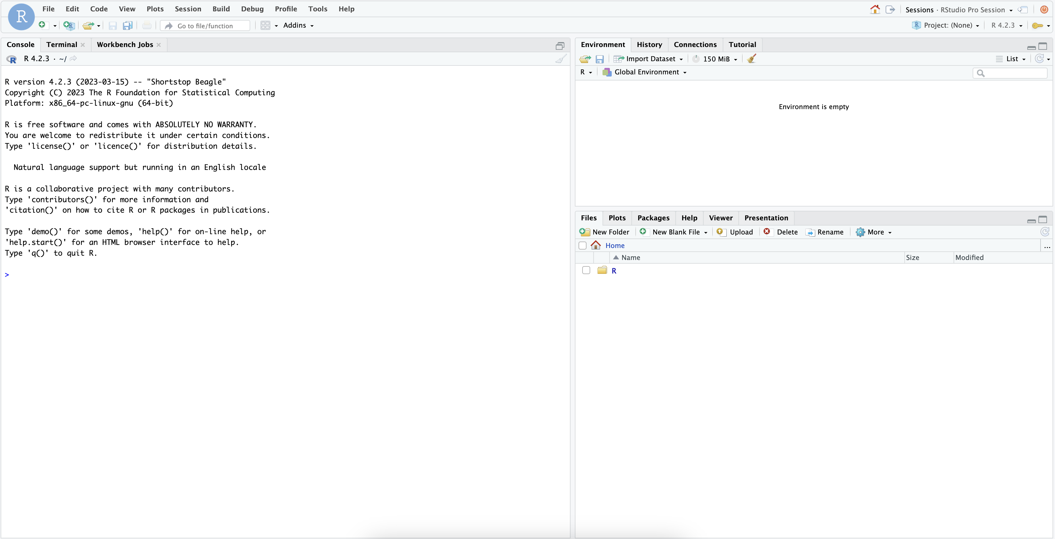
Click Start Session to launch the RStudio Pro IDE.
Once everything is ready, you will be able to work with your Snowflake data in the familiar RStudio Pro IDE. Since the IDE is provided by the Posit Workbench Native App, your entire analysis will run securely within Snowflake.
Step 5: Access the Quickstart Materials
This Quickstart will walk you through the code contained in https://github.com/posit-dev/snowflake-posit-quickstart-orbital/blob/main/fit_and_deploy.R. To follow along, open the file in your RStudio Pro IDE. There are two ways to do this:
- Simple copy-and-paste Go to File > New File > R Script and then copy the contents of fit_and_deploy.R into your new file.
- Starting a new project linked to the GitHub repo. To do this:
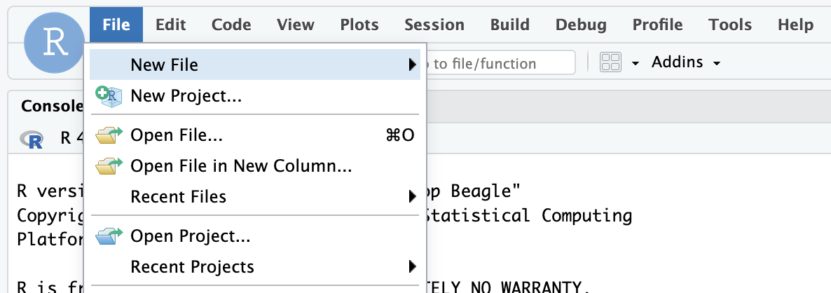
- Go to
File>New Projectin the RStudio IDE menu bar.
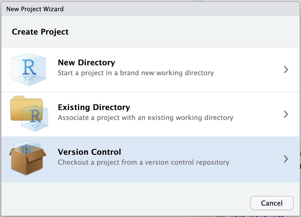
- Select Version Control in the New Project Wizard
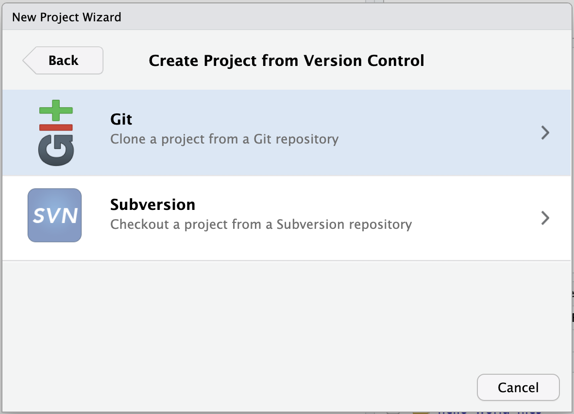
- Select Git
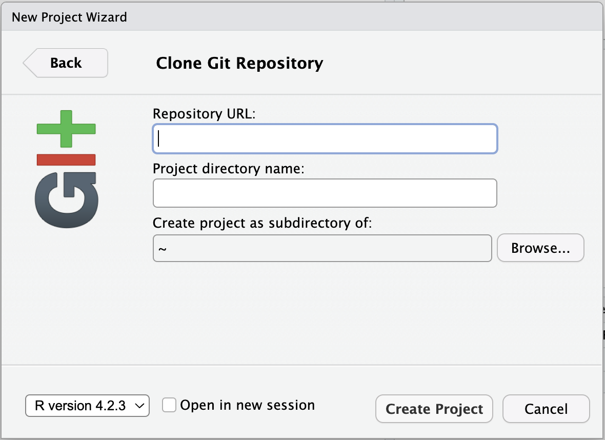
- Paste the URL of the GitHub repo and click Create Project
 RStudio will clone a local copy of the materials on GitHub. You can use the Files pane in the bottom right-hand corner of the IDE to navigate to
 quarto.qmd. Click on the file to open it. - Go to
SSH authentication is not available in Snowpark Container Services, so when creating projects from Git, you may need to authenticate Git operations over HTTPS, using a username and password or a personal access token.
Install R Packages
Now that we're in a familiar R environment, we need to install the necessary packages. We'll use the tidymodels ecosystem of packages, as well as a few others.
install.packages(
  c(
    "odbc",
    "DBI",
    "dbplyr",
    "dplyr",
    "glue",
    "arrow",
    "stringr",
    "tidymodels",
    "vetiver",
    "rsconnect",
    "pins",
    "orbital",
    "tidypredict",
    "ggplot2"
  )
)
After we install the packages, we load them.
library(odbc)
library(DBI)
library(dbplyr)
library(dplyr)
library(glue)
library(arrow)
library(stringr)
library(tidymodels)
library(vetiver)
library(rsconnect)
library(pins)
library(orbital)
library(tidypredict)
library(ggplot2)
Before starting the modeling process, we need to connect to our database and load the loan data.
We'll use the DBI and odbc R packages to connect to the database. We'll then use dplyr and dbplyr to query the data with R without having to write raw SQL. To learn more, see Analyze Data with R using Posit Workbench and Snowflake.
Connect with DBI
First, we use DBI::dbConnect() to connect to Snowflake. We'll also need a driver provided by the odbc package. The warehouse, database, and schema arguments specify our desired Snowflake warehouse, database, and schema.
con <- dbConnect(
  odbc::snowflake(),
  warehouse = "DEFAULT_WH",
  database = "LENDING_CLUB",
  schema = "ML"
)
You may need to change warehouse, database, and schema to match your environment.
con now stores our Snowflake connection.
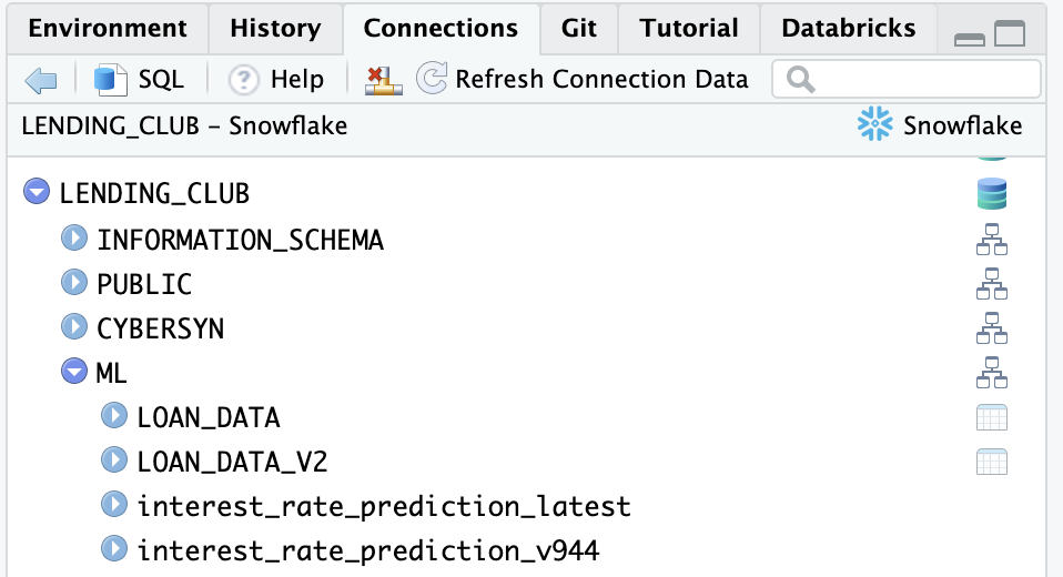
Once connected, we can view available databases, schemas, and tables in the RStudio IDE Connections pane. Click on the database icon to the right of a database to see its schemas. Click on the schema icon to the right of a schema to see its tables. Click the table icon to preview the table.
Create and Manipulate a tbl
Once we build a connection, we can use dplyr::tbl() to create tbls. A tbl is an R object that represents a table or view accessed through a connection.
con |> tbl("LOAN_DATA")
We can also use dbplyr to translate typical dplyr verbs into SQL. To prepare our tbl for modeling, we'll extract the year and month information from the ISSUE_D column.
lendingclub_dat <-
  con |>
  tbl("LOAN_DATA") |>
  mutate(
    ISSUE_YEAR = as.integer(str_sub(ISSUE_D, start = 5)),
    ISSUE_MONTH = as.integer(
      case_match(
        str_sub(ISSUE_D, end = 3),
        "Jan" ~ 1,
        "Feb" ~ 2,
        "Mar" ~ 3,
        "Apr" ~ 4,
        "May" ~ 5,
        "Jun" ~ 6,
        "Jul" ~ 7,
        "Aug" ~ 8,
        "Sep" ~ 9,
        "Oct" ~ 10,
        "Nov" ~ 11,
        "Dec" ~ 12
      )
    )
  )
We don't want to fit our model on all 2.3 million rows, so we'll filter to a single year and then sample 5,000 rows.
lendingclub_sample <-
  lendingclub_dat |>
  filter(ISSUE_YEAR == 2016) |>
  slice_sample(n = 5000)
Our ultimate goal is to create a model that predicts loan interest rates (the INT_RATE column). To prepare our data for modeling, we'll first select a few columns of interest (loan term, credit utilization, credit open-to-buy, and all utilization), convert INT_RATE to a numeric variable, and remove missing values.
lendingclub_prep <-
  lendingclub_sample |>
  select(INT_RATE, TERM, BC_UTIL, BC_OPEN_TO_BUY, ALL_UTIL) |>
  mutate(INT_RATE = as.numeric(str_remove(INT_RATE, "%"))) |>
  filter(!if_any(everything(), is.na)) |>
  collect()
collect() executes a query and returns the entire result as a tibble, so lendingclub_prep now contains our entire filtered sample.
Create a Workflow
Next, we'll create a tidymodels workflow. Workflows bundle pre-processing, modeling, and post-processing steps. Learn more about workflows here.
The first step is to specify our model formula and pre-processing steps using the recipes package.
# Pre-processing
lendingclub_rec <-
  recipe(INT_RATE ~ ., data = lendingclub_prep) |>
  step_mutate(TERM = (TERM == "60 months")) |>
  step_mutate(across(!TERM, as.numeric)) |>
  step_normalize(all_numeric_predictors()) |>
  step_impute_mean(all_of(c("BC_OPEN_TO_BUY", "BC_UTIL"))) |>
  step_filter(!if_any(everything(), is.na))
Our recipe lendingclub_rec defines our model formula: we'll use all the other variables in the dataset to predict the interest rate. We also perform a few pre-processing steps, including turning TERM into a logical, normalizing all numeric predictors, and removing missing values.
Next, we define the type of model we want to fit: a linear model. linear_reg() is from the parsnip package.
lendingclub_lr <- linear_reg()
Now, we can create our workflow, adding our linear model and pre-processing recipe.
lendingclub_wf <-
  workflow() |>
  add_model(lendingclub_lr) |>
  add_recipe(lendingclub_rec)
Our workflow object now looks like this:
lendingclub_wf
══ Workflow ═══════════════════════════════════════════════════════════════════════════════════════════════════════
Preprocessor: Recipe
Model: linear_reg()

── Preprocessor ───────────────────────────────────────────────────────────────────────────────────────────────────
5 Recipe Steps

• step_mutate()
• step_mutate()
• step_normalize()
• step_impute_mean()
• step_filter()

── Model ──────────────────────────────────────────────────────────────────────────────────────────────────────────
Linear Regression Model Specification (regression)

Computational engine: lm
Notice that it includes our pre-processing steps and model specification.
Fit Model and Compute Metrics
Now that we have our workflow object lendingclub_wf, we can use it to fit our model.
lendingclub_fit <-
  lendingclub_wf |>
  fit(data = lendingclub_prep)
To understand how well our model performs, we define a metric set using yardstick::metric_set() and then compute those metrics for lendingclub_fit.
lendingclub_metric_set <- metric_set(rmse, mae, rsq)

lendingclub_metrics <-
  lendingclub_fit |>
  augment(lendingclub_prep) |>
  lendingclub_metric_set(truth = INT_RATE, estimate = .pred)
lendingclub_metrics looks like this:
# A tibble: 3 × 3
  .metric .estimator .estimate
  <chr>   <chr>          <dbl>
1 rmse    standard       4.38
2 mae     standard       3.43
3 rsq     standard       0.233
Version Model with vetiver
The vetiver package provides tools to version, share, deploy, and monitor models.
We'll use vetiver to version and write our fitted model to a pin on Posit Connect. This will allow us to identify which version of our model is active and track performance against other models over time.
First, we need to connect to a Posit Connect board.
board <- board_connect()
To run rsconnect::board_connect(), you'll first need to authenticate. To authenticate, navigate to Tools > Global Options > Publishing > Connect and follow the instructions.
Then, we create a vetiver model with vetiver_model(), supplying the function with our fitted model, model name, and metadata containing our metrics.
model_name <- "interest_rate_prediction"
v <-
  vetiver_model(
    lendingclub_fit,
    model_name,
    metadata = list(metrics = lendingclub_metrics)
  )
vetiver_pin_write() writes the vetiver model to Posit Connect as a pin.
board |> vetiver_pin_write(v)
If you run into a namespacing error in Connect, or a permissioning error in Snowflake, that may mean someone has already run this code with the same model_name. You'll need to pick a different value.
We can use pin_versions() to return all the different versions of this model.
model_versions <-
  board |>
  pin_versions(glue("{board$account}/{model_name}"))
Unless you've done this Quickstart multiple times, you'll probably only have one model version.
Let's grab the active version of the model. We'll use this later when interacting with Snowflake.
model_version <-
  model_versions |>
  filter(active) |>
  pull(version)
At this point, we've:
- Fit a model
- Evaluated that model
- Versioned the model with vetiver
- Stored the model as a pin on Posit Connect
Now, we're ready to deploy the model with orbital and Snowflake.
The orbital package allows you to run tidymodels workflow predictions inside databases, including Snowflake, substantially speeding up the prediction process.
To do so, orbital converts tidymodels workflows into SQL that can run on Snowflake. You can then either use that SQL to run the predictions of that model or deploy the model directly to Snowflake as a view.
Convert Workflow to orbital
Let's convert our tidymodels object into an orbital object with orbital().
orbital_obj <- orbital(lendingclub_fit)
orbital_obj
── orbital Object ─────────────────────────────────────────────────────────────────────────────────────────────────
• TERM = (TERM == "60 months")
• BC_UTIL = (BC_UTIL - 58.37713) / 27.86179
• BC_OPEN_TO_BUY = (BC_OPEN_TO_BUY - 10906.02) / 16427.05
• ALL_UTIL = (ALL_UTIL - 60.11253) / 20.41787
• BC_OPEN_TO_BUY = dplyr::if_else(is.na(BC_OPEN_TO_BUY), 2.678412e-17, BC_OPEN_TO_BUY)
• BC_UTIL = dplyr::if_else(is.na(BC_UTIL), 2.691542e-17, BC_UTIL)
• .pred = 11.96049 + (ifelse(TERM == "TRUE", 1, 0) * 4.308234) + (BC_UTIL * 0.1679237) + (BC_OPEN_TO_BUY * - ...
───────────────────────────────────────────────────────────────────────────────────────────────────────────────────
7 equations in total.
If you want to see the SQL statement generated by the model, run orbital_sql().
sql_predictor <- orbital_sql(orbital_obj, con)
sql_predictor
<SQL> ("TERM" = '60 months') AS TERM
<SQL> ("BC_UTIL" - 58.3771301356001) / 27.8617927834219 AS BC_UTIL
<SQL> ("BC_OPEN_TO_BUY" - 10906.0174053835) / 16427.0528247826 AS BC_OPEN_TO_BUY
<SQL> ("ALL_UTIL" - 60.1125278283748) / 20.4178686256935 AS ALL_UTIL
<SQL> CASE WHEN (("BC_OPEN_TO_BUY" IS NULL)) THEN 2.67841164255808e-17 WHEN NOT (("BC_OPEN_TO_BUY" IS NULL)) THEN "BC_OPEN_TO_BUY" END AS BC_OPEN_TO_BUY
<SQL> CASE WHEN (("BC_UTIL" IS NULL)) THEN 2.69154231610625e-17 WHEN NOT (("BC_UTIL" IS NULL)) THEN "BC_UTIL" END AS BC_UTIL
<SQL> (((11.9604886671368 + (CASE WHEN ("TERM" = 'TRUE') THEN 1.0 WHEN NOT ("TERM" = 'TRUE') THEN 0.0 END * 4.30823403045859)) + ("BC_UTIL" * 0.167923700948935)) + ("BC_OPEN_TO_BUY" * -0.892522593408621)) + ("ALL_UTIL" * 0.684415441909473) AS .pred
Notice that you can see all the pre-processing steps and model prediction steps.
Run predictions in Snowflake
Now that we've converted our tidymodels workflow object to SQL with orbital, we can run model predictions inside Snowflake.
Calling predict() with our orbital object will run the SQL code we saw above directly in Snowflake.
start_time <- Sys.time()
preds <-
  predict(orbital_obj, lendingclub_dat) |>
  compute(name = "LENDING_CLUB_PREDICTIONS_TEMP")

end_time <- Sys.time()

preds
# Source:   SQL [?? x 1]
# Database: Snowflake 8.44.2[@Snowflake/LENDING_CLUB]
   .pred
   <dbl>
 1  13.6
 2  17.0
 3  12.5
 4  13.6
 5  11.9
 6  16.8
 7  12.3
 8  11.3
 9  14.0
10  13.5
# ℹ more rows
# ℹ Use `print(n = ...)` to see more rows
We've also used dplyr::compute() to force the query to compute—without compute(), predict() would only be evaluated lazily. compute() saves the results to a temporary table. The Sys.time() calls will help us determine how fast orbital computed our predictions.
To figure out how much orbital sped up our process, let's see how many predictions we computed:
preds |> count()
# Source:   SQL [1 x 1]
# Database: Snowflake 8.44.2[@Snowflake/LENDING_CLUB]
        n
    <dbl>
1 2260702
as well as how much time elapsed:
end_time - start_time
Time difference of 3.027164 secs
2,260,702 predictions in just 3.02 seconds—thanks to Snowflake and orbital!
Next, we'll deploy our model so others can use it. We have a couple of options.
One option is to write the predictions back to Snowflake as a permanent table by setting temporary = FALSE in compute():
preds <-
  predict(orbital_obj, lendingclub_dat) |>
  compute(name = "LENDING_CLUB_PREDICTIONS", temporary = FALSE)
Another is to write our model prediction function as a view.
To create this view, we first need to construct the SQL query that we want to store in the view.
view_sql <-
  lendingclub_dat |>
  mutate(!!!orbital_inline(orbital_obj)) |>
  select(any_of(c("ID", ".pred"))) |>
  remote_query()
orbital_inline() allows us to use our orbital object in a dplyr pipeline. We can then use select() to select just the columns we need for our predictions view: ID (to identify the rows) and .pred (which contains the predictions).
dbplyr::remote_query() converts our dplyr pipeline back into SQL. Let's take a look at the result.
view_sql
<SQL> SELECT
  "ID",
  (((11.8433051541854 + (CASE WHEN ("TERM" = 'TRUE') THEN 1.0 WHEN NOT ("TERM" = 'TRUE') THEN 0.0 END * 4.38875098270329)) + ("BC_UTIL" * -0.083097744438186)) + ("BC_OPEN_TO_BUY" * -0.894697830285346)) + ("ALL_UTIL" * 0.743982590927869) AS ".pred"
FROM (
  SELECT
    "ID",
    "MEMBER_ID",
    "LOAN_AMNT",
    ...
    "ACC_OPEN_PAST_24MTHS",
    "AVG_CUR_BAL",
    CASE WHEN (("BC_OPEN_TO_BUY" IS NULL)) THEN 2.4581101886311e-17 WHEN NOT (("BC_OPEN_TO_BUY" IS NULL)) THEN "BC_OPEN_TO_BUY" END AS "BC_OPEN_TO_BUY",
    CASE WHEN (("BC_UTIL" IS NULL)) THEN 9.95071097045741e-17 WHEN NOT (("BC_UTIL" IS NULL)) THEN "BC_UTIL" END AS "BC_UTIL",
    "CHARGEOFF_WITHIN_12_MTHS",
    "DELINQ_AMNT",
    "MO_SIN_OLD_IL_ACCT",
    "MO_SIN_OLD_REV_TL_OP",
    "MO_SIN_RCNT_REV_TL_OP",
    ...
    "ISSUE_MONTH"
  FROM (
    SELECT
      "ID",
      "MEMBER_ID",
      "LOAN_AMNT",
      "FUNDED_AMNT",
      "FUNDED_AMNT_INV",
      ...
      "SETTLEMENT_TERM",
      "ISSUE_YEAR",
      "ISSUE_MONTH"
    FROM (
      SELECT
        "LOAN_DATA".*,
        CAST(SUBSTR("ISSUE_D", 5) AS INT) AS "ISSUE_YEAR",
        CAST(CASE
WHEN (SUBSTR("ISSUE_D", 1, 3) IN ('Jan')) THEN 1.0
...
WHEN (SUBSTR("ISSUE_D", 1, 3) IN ('Dec')) THEN 12.0
END AS INT) AS "ISSUE_MONTH"
      FROM "LOAN_DATA"
    ) "q01"
  ) "q01"
) "q01"
We've abbreviated the query here for brevity.
This SQL query uses our model to compute a predicted value for each loan in the LOAN_DATA table. It creates a table with two columns, ID and .PRED, which are all we need when creating a table of predictions. Later, if someone wants to use our prediction table, they can use the ID column to join the predictions back to the loan data.
Now, we'll take this SQL and create a view. First, we create a name for our view by glueing together the model name and version.
versioned_view_name <- glue("{model_name}_v{model_version}")
Then, we use glue_sql() to combine the SQL needed to create a view with our model prediction SQL from above.
snowflake_view_statement <-
  glue_sql(
    "CREATE OR REPLACE VIEW {`versioned_view_name`} AS ",
    view_sql,
    .con = con
  )
Finally, we execute this complete SQL query with DBI::dbExecute().
con |>
  DBI::dbExecute(snowflake_view_statement)
[1] 0
dbExecute() returned 0 because it returns the number of rows changed. We created a new view, so we changed 0 rows.
Our view is now in Snowflake and ready to use!
Create a Latest View
So far, we've only created one view for our one model version. But what if you have multiple views corresponding to multiple versions of your model? It would be helpful to have a view that always corresponds to the latest version of the model. Let's make that view.
First, we'll make a name for this new view.
main_view_name <- glue::glue("{model_name}_latest")
Then, we again use glue_sql() and dbExecute() to create the view.
main_view_statement <- glue::glue_sql(
  "CREATE OR REPLACE VIEW {`main_view_name`} AS ",
  "SELECT * FROM {`versioned_view_name`}",
  .con = con
)

con |>
  DBI::dbExecute(main_view_statement)
We can take a look at this view using tbl() and collect() to pull the view into R.
con |>
  tbl(main_view_name) |>
  head(100) |>
  collect()
# A tibble: 100 × 2
   ID        .pred
   <chr>     <dbl>
 1 142212962 16.7
 2 142529846 12.4
 3 141649517 13.7
 4 141671381 13.1
 5 141449070 16.9
 6 142661219 11.6
 7 142647391 15.9
 8 142646325  8.37
 9 142211815  9.98
10 142661174 11.1
# ℹ 90 more rows
# ℹ Use `print(n = ...)` to see more rows
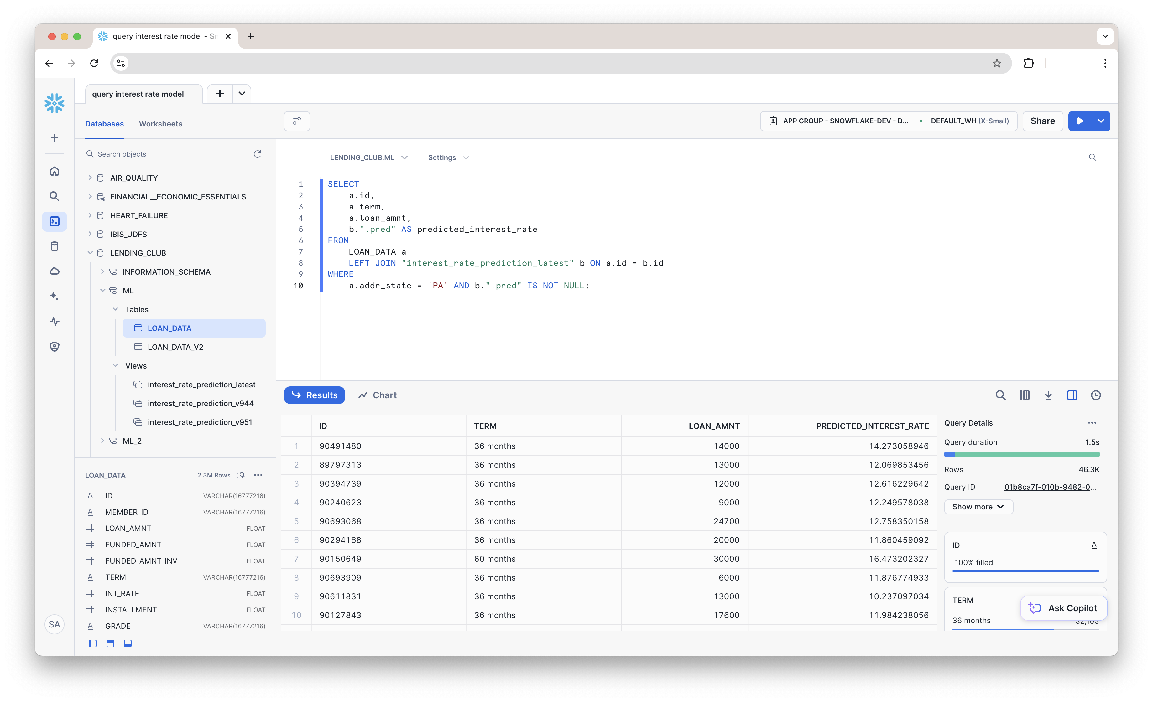
Now, we have a table of predictions we can share with others in our organization through Snowflake. They can use our view no matter what tools they're using to interact with Snowflake, including Snowsight, as shown below.
As new data comes in over time, it is useful to refit our model. We can refit periodically, monitor performance, and store the best-performing version on Posit Connect. We won't cover this in detail here, but we've put together sample code for the process in this Quarto document.
This blog post also covers the process.
Conclusion
In this Quickstart, you learned how to use orbital and tidymodels to build, deploy, and run predictions directly in Snowflake. By combining the power of Snowflake with the flexibility of R, you can efficiently scale your modeling workflows and share results as views, all within a secure environment.
What You Learned
- How to use the Posit Workbench Native App to interact with Snowflake from the RStudio IDE.
- How to create a tidymodels workflow with the recipes and workflows packages.
- How to use vetiver to version models and store them as pins on Posit Connect.
- How to use orbital package to convert tidymodels workflows into SQL and run predictions directly inside Snowflake.
- How to deploy predictions as Snowflake views.