AI-powered Business Intelligence (BI) and conversational analytics hold immense promise for data-driven decision-making. However, directly applying these technologies to complex enterprise schemas often leads to inaccurate or inconsistent results, commonly referred to as "hallucinations." This challenge arises because AI and BI systems may struggle to interpret raw data without a clear understanding of the organizational context and definitions.
Snowflake addresses these challenges by introducing Semantic Views, a new schema-level object that stores all semantic model information natively within the database. Semantic views capture and store semantic model information directly within the database, including business-relevant concepts such as metrics (e.g., total sales), dimensions (e.g., product category), and facts.
What You'll Learn
- How to setup a database and schema in Snowflake
- How to create views from existing sample data
- The process of defining a Snowflake semantic view with tables, relationships, dimensions, and metrics
- How to query a semantic view
- How semantic views enhance AI-powered analytics and consistency across BI tools
What You'll Build
You will build a foundational understanding and practical setup of a Snowflake semantic view, complete with data views and a defined semantic model, enabling simplified and consistent data querying for BI and AI applications using TPC-DS sample data.
What You'll Need
- Access to a Snowflake account
- Basic knowledge of SQL and Python
- Familiarity with data analysis concepts
- Access to
ACCOUNTADMINrole is required for creating semantic views) - Access to the
SNOWFLAKE_SAMPLE_DATAdatabase
What is a Semantic View?
A semantic view acts as a translator between your raw data and how humans or AI interpret it. It defines key business concepts like "metrics" (e.g., total sales) and "dimensions" (e.g., customer location) by referencing your underlying tables and their relationships.
Why Semantic Views Matter
Semantic views are crucial for several reasons:
- Ensures AI and BI consistency: By embedding organizational context and definitions directly into the data layer, semantic views ensure that both AI and BI systems interpret information uniformly, leading to trustworthy answers.
- Enables AI-powered analytics: They make data "AI-ready," unlocking advanced use cases such as conversational analytics and significantly reducing the risk of AI hallucinations.
- Maintains consistency across BI Tools: Semantic models are shifted from individual BI tool layers to the core data platform, guaranteeing that all tools utilize the same semantic concepts.
- Unlocks rich analytical capabilities: Semantic views power diverse user interfaces, including AI-powered analytics, traditional BI clients, Streamlit applications, and custom applications.
Basic Elements of a Semantic View Definition
Every semantic view definition requires essential elements:
- Physical model objects: These refer to your existing tables, views, or (in future releases) SQL queries that contain the raw data.
- Relationships: These define how your physical objects connect to each other (e.g., a CUSTOMER table linked to an ORDERS table).
- Dimensions: These are business-friendly attributes used to group or filter your data (e.g., customer's birth year, product category).
- Metrics: These are business-friendly calculations or aggregations, often representing Key Performance Indicators (KPIs) (e.g., total sales price, total sales quantity).
Download the Notebook
Firstly, to follow along with this quickstart, you can click on getting-started-with-snowflake-semantic-view.ipynb to download the Notebook from GitHub.
Snowflake Notebooks come pre-installed with common Python libraries for data science and machine learning, such as numpy, pandas, matplotlib, and more! If you are looking to use other packages, click on the Packages dropdown on the top right to add additional packages to your notebook.
Setup your Database and Schema
First, we'll create a new database named SAMPLE_DATA and a schema named TPCDS_SF10TCL to organize our data. We will then set the context to use this new schema.
-- Create a new test database named SAMPLE_DATA
CREATE DATABASE SAMPLE_DATA;

-- Use the newly created database
USE DATABASE SAMPLE_DATA;

-- Create a new schema named TPCDS_SF10TCL within SAMPLE_DATA
CREATE SCHEMA TPCDS_SF10TCL;

-- Set the context to use the new schema
USE SCHEMA TPCDS_SF10TCL;
Create Views from Sample Data
Next, we'll create views for the tables we want to analyze. These views will be based on the SNOWFLAKE_SAMPLE_DATA.TPCDS_SF10TCL dataset, allowing us to work with a subset of the data without modifying the original tables.
-- Create or replace views for the tables from SNOWFLAKE_SAMPLE_DATA.TPCDS_SF10TCL

CREATE OR REPLACE VIEW CUSTOMER AS
SELECT * FROM SNOWFLAKE_SAMPLE_DATA.TPCDS_SF10TCL.CUSTOMER;

CREATE OR REPLACE VIEW CUSTOMER_DEMOGRAPHICS AS
SELECT * FROM SNOWFLAKE_SAMPLE_DATA.TPCDS_SF10TCL.CUSTOMER_DEMOGRAPHICS;

CREATE OR REPLACE VIEW DATE_DIM AS
SELECT * FROM SNOWFLAKE_SAMPLE_DATA.TPCDS_SF10TCL.DATE_DIM;

CREATE OR REPLACE VIEW ITEM AS
SELECT * FROM SNOWFLAKE_SAMPLE_DATA.TPCDS_SF10TCL.ITEM;

CREATE OR REPLACE VIEW STORE AS
SELECT * FROM SNOWFLAKE_SAMPLE_DATA.TPCDS_SF10TCL.STORE;

CREATE OR REPLACE VIEW STORE_SALES AS
SELECT * FROM SNOWFLAKE_SAMPLE_DATA.TPCDS_SF10TCL.STORE_SALES;
Verify your Environment Setup
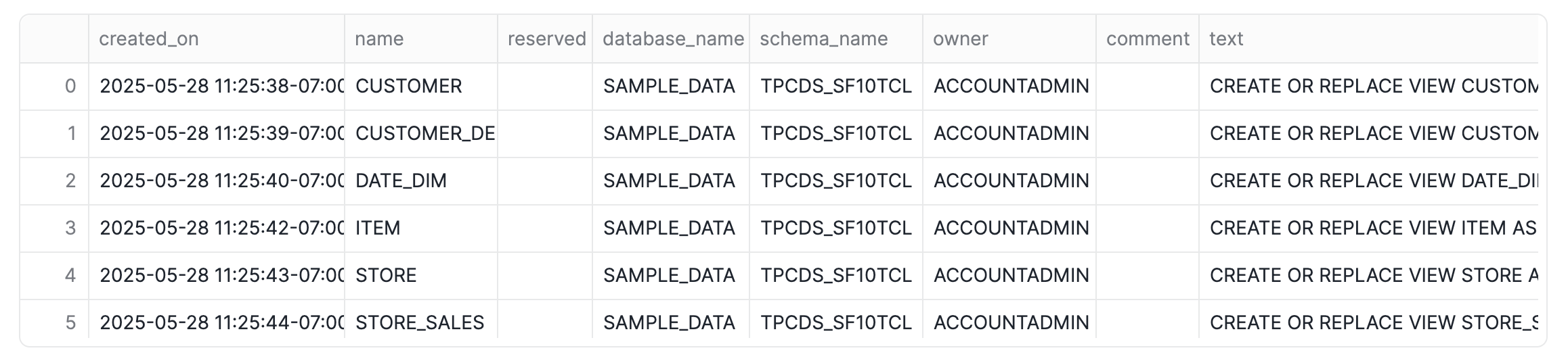
Before proceeding, let's ensure our warehouse, database, and schema are correctly set, and then list the views we just created.
-- Select the warehouse, database, and schema
USE WAREHOUSE COMPUTE_WH;
USE DATABASE SAMPLE_DATA;
USE SCHEMA TPCDS_SF10TCL;

-- Show all views in the current schema to verify creation
SHOW VIEWS;
Define the Semantic View
We'll start by switching to the ACCOUNTADMIN role:
-- Switch to ACCOUNTADMIN role to create the semantic view
USE ROLE ACCOUNTADMIN;
Now, we'll define our TPCDS_SEMANTIC_VIEW_SM semantic view. This view will establish relationships between our tables, define facts (measures), and dimensions (attributes), making it easier to query and analyze our data without complex joins.
-- Create or replace the semantic view named TPCDS_SEMANTIC_VIEW_SM
CREATE OR REPLACE SEMANTIC VIEW TPCDS_SEMANTIC_VIEW_SM
	tables (
		CUSTOMER primary key (C_CUSTOMER_SK),
		DATE as DATE_DIM primary key (D_DATE_SK),
		DEMO as CUSTOMER_DEMOGRAPHICS primary key (CD_DEMO_SK),
		ITEM primary key (I_ITEM_SK),
		STORE primary key (S_STORE_SK),
		STORESALES as STORE_SALES
        primary key (SS_SOLD_DATE_SK,SS_CDEMO_SK,SS_ITEM_SK,SS_STORE_SK,SS_CUSTOMER_SK)
	)
	relationships (
		SALESTOCUSTOMER as STORESALES(SS_CUSTOMER_SK) references CUSTOMER(C_CUSTOMER_SK),
		SALESTODATE as STORESALES(SS_SOLD_DATE_SK) references DATE(D_DATE_SK),
		SALESTODEMO as STORESALES(SS_CDEMO_SK) references DEMO(CD_DEMO_SK),
		SALESTOITEM as STORESALES(SS_ITEM_SK) references ITEM(I_ITEM_SK),
		SALETOSTORE as STORESALES(SS_STORE_SK) references STORE(S_STORE_SK)
	)
	facts (
		ITEM.COST as i_wholesale_cost,
		ITEM.PRICE as i_current_price,
		STORE.TAX_RATE as S_TAX_PRECENTAGE,
        STORESALES.SALES_QUANTITY as SS_QUANTITY
	)
	dimensions (
		CUSTOMER.BIRTHYEAR as C_BIRTH_YEAR,
		CUSTOMER.COUNTRY as C_BIRTH_COUNTRY,
		CUSTOMER.C_CUSTOMER_SK as c_customer_sk,
		DATE.DATE as D_DATE,
		DATE.D_DATE_SK as d_date_sk,
		DATE.MONTH as D_MOY,
		DATE.WEEK as D_WEEK_SEQ,
		DATE.YEAR as D_YEAR,
		DEMO.CD_DEMO_SK as cd_demo_sk,
		DEMO.CREDIT_RATING as CD_CREDIT_RATING,
		DEMO.MARITAL_STATUS as CD_MARITAL_STATUS,
		ITEM.BRAND as I_BRAND,
		ITEM.CATEGORY as I_CATEGORY,
		ITEM.CLASS as I_CLASS,
		ITEM.I_ITEM_SK as i_item_sk,
		STORE.MARKET as S_MARKET_ID,
		STORE.SQUAREFOOTAGE as S_FLOOR_SPACE,
		STORE.STATE as S_STATE,
		STORE.STORECOUNTRY as S_COUNTRY,
		STORE.S_STORE_SK as s_store_sk,
		STORESALES.SS_CDEMO_SK as ss_cdemo_sk,
		STORESALES.SS_CUSTOMER_SK as ss_customer_sk,
		STORESALES.SS_ITEM_SK as ss_item_sk,
		STORESALES.SS_SOLD_DATE_SK as ss_sold_date_sk,
		STORESALES.SS_STORE_SK as ss_store_sk
	)
	metrics (
		STORESALES.TOTALCOST as SUM(item.cost),
		STORESALES.TOTALSALESPRICE as SUM(SS_SALES_PRICE),
		STORESALES.TOTALSALESQUANTITY as SUM(SS_QUANTITY)
            WITH SYNONYMS = ( 'total sales quantity', 'total sales amount')
	)

;
Verify the Semantic View Creation
Let's confirm that our semantic view has been successfully created by listing all semantic views in the current database.
-- Lists semantic views in the database that is currently in use
SHOW SEMANTIC VIEWS;

Describe the Semantic View
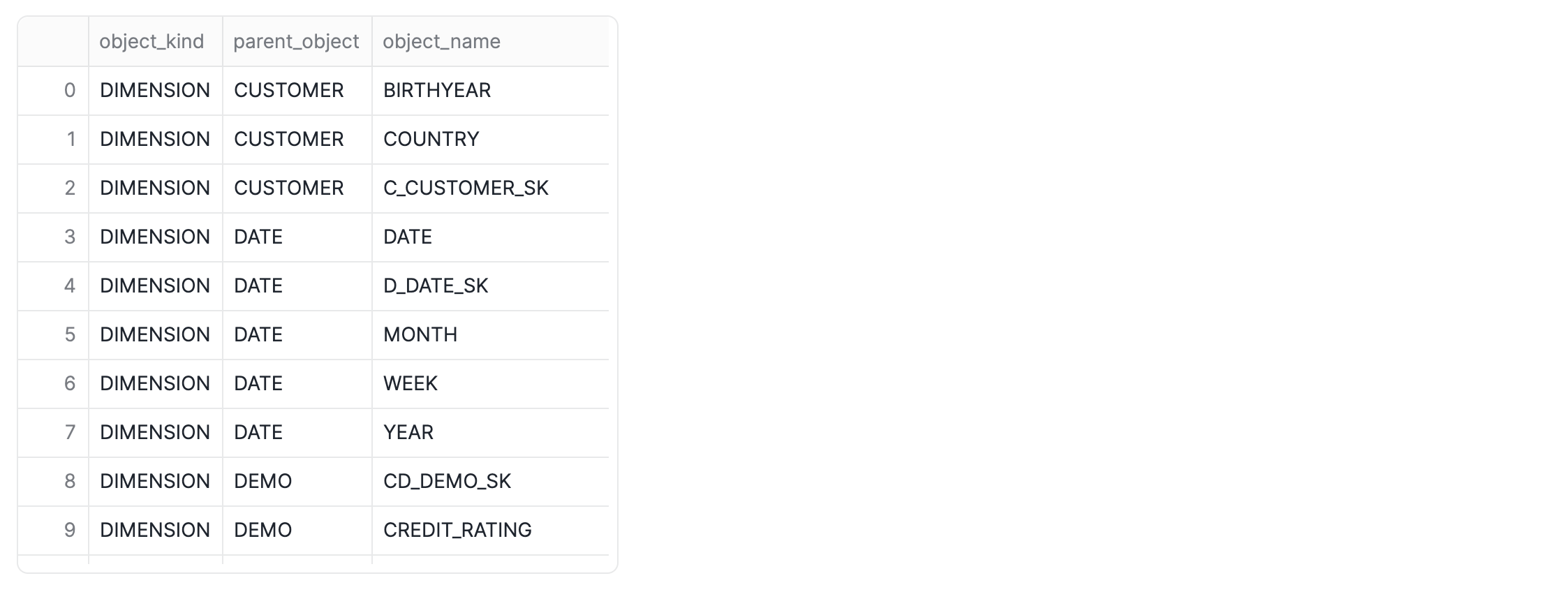
To understand the structure and components of our newly created semantic view, we can use the DESC SEMANTIC VIEW command. This will provide details about its tables, relationships, facts, and dimensions.
-- Describes the semantic view named TPCDS_SEMANTIC_VIEW_SM, and as a special bonus uses our new flow operator to filter and project only the metric and dimension names

DESC SEMANTIC VIEW TPCDS_SEMANTIC_VIEW_SM
    ->> SELECT "object_kind","property_value" as "parent_object","object_name" FROM $1
        WHERE "object_kind" IN ('METRIC','DIMENSION') AND "property" IN ('TABLE')
;
Natural Language Querying
Snowflake's Cortex Analyst allows you to interact with your semantic views using natural language. This powerful feature transforms how users can explore data without needing to know SQL syntax.
Access Cortex Analyst
You can access Cortex Analyst through the Snowflake interface.
Let's dynamically generate a link to Cortex Analyst so that you can access the semantic view.
First, we'll create a SQL cell named sql_step7:
SELECT 'https://app.snowflake.com/' || CURRENT_ORGANIZATION_NAME() || '/' || CURRENT_ACCOUNT_NAME() || '/#/studio/analyst/databases/SAMPLE_DATA/schemas/TPCDS_SF10TCL/semanticView/TPCDS_SEMANTIC_VIEW_SM/edit' AS RESULT;
Next, we'll call it from the following Python code cell that we called py_link:
import streamlit as st

link = sql_step7.to_pandas()['RESULT'].iloc[0]

st.link_button("Go to Cortex Analyst", link)
Example Natural Language Query
Once in Cortex Analyst, you can ask questions like:
Show me the top selling brands in by total sales quantity in the state ‘TX' in the ‘Books' category in the year 2003
Cortex Analyst will automatically translate this natural language question into the appropriate Semantic SQL query and return the results.
Basic Query Structure
To query a semantic view, you'll use this special query structure:
SELECT * FROM SEMANTIC_VIEW (view_name
    METRICS metric1, metric2, ...
    DIMENSIONS dimension1, dimension2, ...
);
Let's break down each part:
SELECT * FROM SEMANTIC_VIEW (view_name ...): This initiates your query, indicating that you want to retrieve data from a semantic viewMETRICS metric1, metric2, ...: Within the parentheses, specify the metrics (calculated values or totals) you wish to retrieveDIMENSIONS dimension1, dimension2, ...: Next, specify the dimensions (categories or attributes) you want to group or filter your data by
Add Filters and Sorting
You can enhance your queries with standard SQL clauses:
- Filtering: Use
WHEREclauses to filter your results - Sorting: Use
ORDER BYto sort your results - Limiting: Use
LIMITto restrict the number of results
Example Query: Top Selling Brands
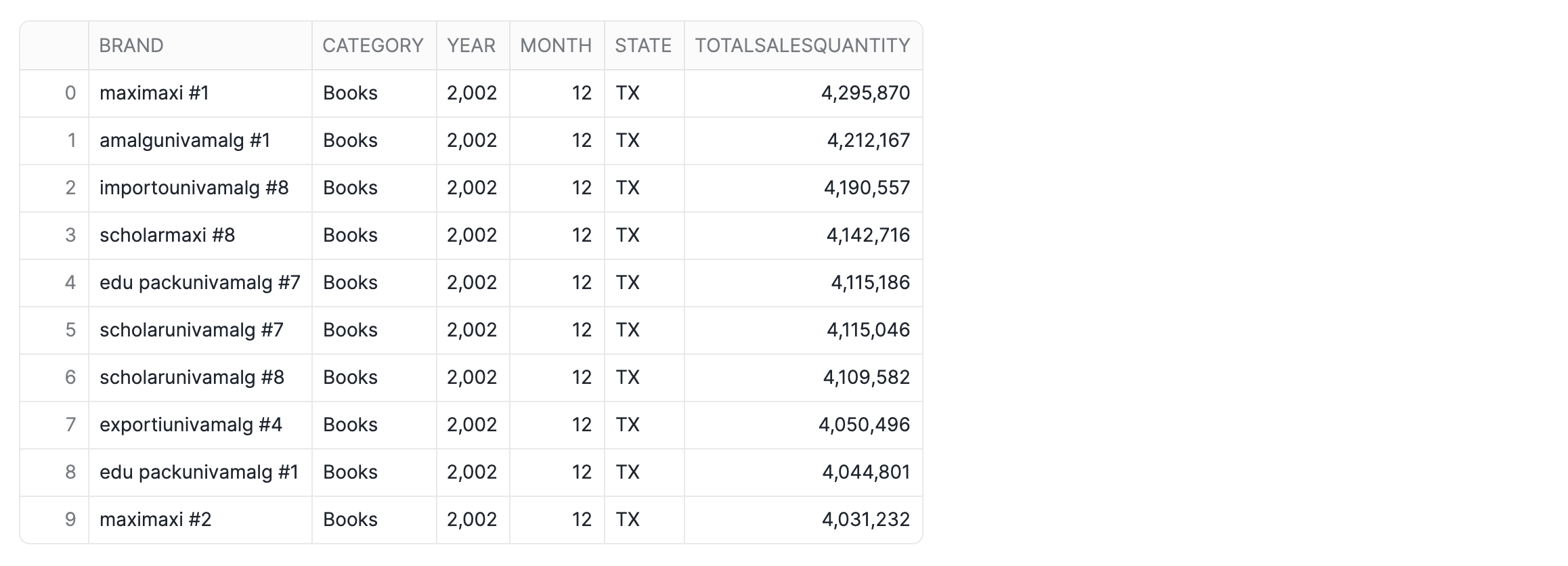
Now that our semantic view is defined, we can easily query it to retrieve aggregated data. The following query demonstrates how to find the top-selling brands in a specific state and category for a given year and month:
-- Query the semantic view to find top selling brands
SELECT * FROM SEMANTIC_VIEW
(
 TPCDS_SEMANTIC_VIEW_SM
    DIMENSIONS
            Item.Brand,
            Item.Category,
            Date.Year,
            Date.Month,
            Store.State
    METRICS
        StoreSales.TotalSalesQuantity
)
WHERE Year = '2002' AND Month = '12' AND State ='TX' AND Category = 'Books'
ORDER BY TotalSalesQuantity DESC LIMIT 10;
In this step, we'll build 2 simple interactive data apps:
- Interactive data visualization app
- Simple interactive dashboard
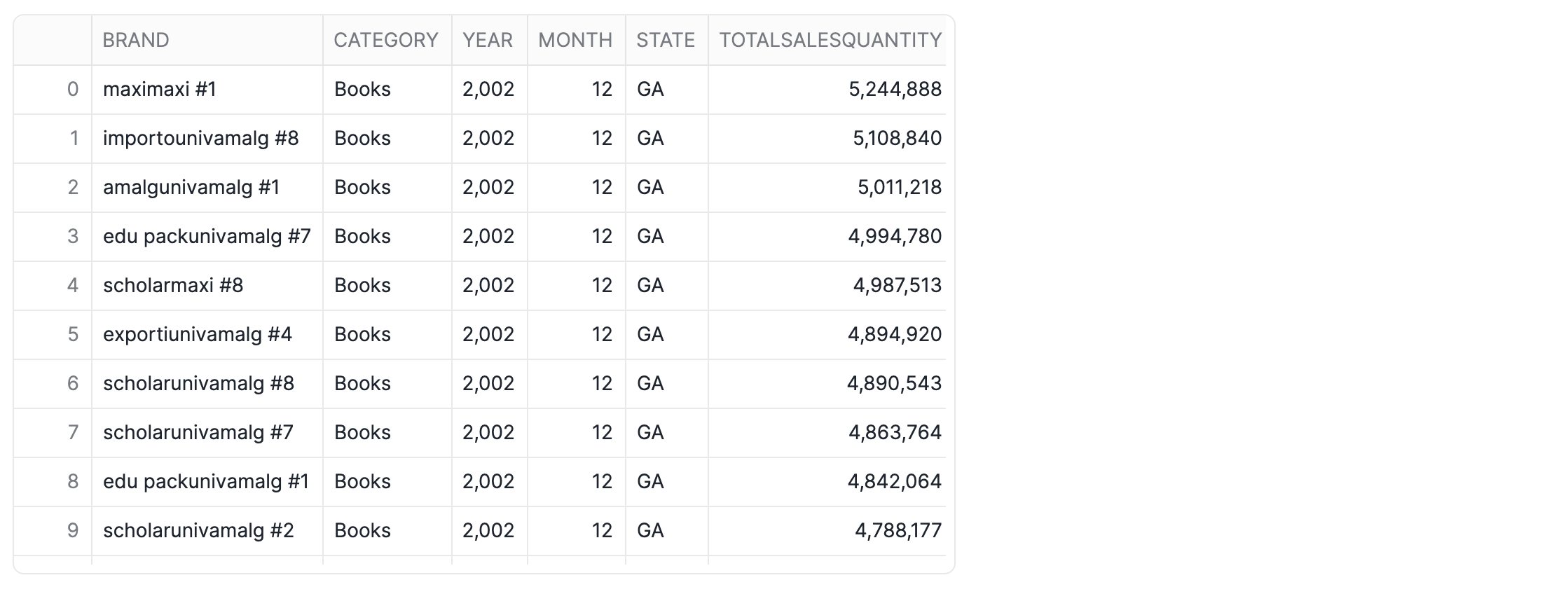
Query data
Firstly, we'll modify the SQL query to show data for month 12.
-- Query the semantic view for month 12
SELECT * FROM SEMANTIC_VIEW
(
 TPCDS_SEMANTIC_VIEW_SM
    DIMENSIONS
            Item.Brand,
            Item.Category,
            Date.Year,
            Date.Month,
            Store.State
    METRICS
        StoreSales.TotalSalesQuantity
    WHERE
        Date.Year = '2002' AND Date.Month = '12' AND Item.Category = 'Books'
)
ORDER BY TotalSalesQuantity DESC;
Next, in a Python cell named df, we'll convert the SQL table to a Pandas DataFrame:
cell1.to_pandas()
App 1: Interactive data visualization app
Here the user can interactively explore the sales data:
import streamlit as st
import pandas as pd

st.title("📊 Sales Data Interactive Visualization")

# Create selectbox for grouping option
group_by = st.selectbox(
    "Select grouping option:",
    options=['BRAND', 'STATE'],
    index=0
)

# Group the data based on selection
if group_by == 'BRAND':
    grouped_data = df.groupby('BRAND')['TOTALSALESQUANTITY'].sum().reset_index()
    grouped_data = grouped_data.set_index('BRAND')
    chart_title = "Total Sales Quantity by Brand"
else:  # group_by == 'STATE'
    grouped_data = df.groupby('STATE')['TOTALSALESQUANTITY'].sum().reset_index()
    grouped_data = grouped_data.set_index('STATE')
    chart_title = "Total Sales Quantity by State"

# Display the chart
st.subheader(chart_title)
st.bar_chart(grouped_data['TOTALSALESQUANTITY'])

# Optional: Display the data table
if st.checkbox("Show data table"):
    st.subheader("Grouped Data")
    st.dataframe(grouped_data)
App 2: Simple interactive dashboard
Here's a simple dashboard we're we've included a row of metrics:
import streamlit as st
import pandas as pd

st.title("📊 Sales Data Dashboard")

# Create selectbox for grouping option
group_by = st.selectbox(
    "Select grouping option:",
    options=['BRAND', 'STATE'],
    index=0
)

# Group the data based on selection
if group_by == 'BRAND':
    grouped_data = df.groupby('BRAND')['TOTALSALESQUANTITY'].sum().reset_index()
    grouped_data = grouped_data.set_index('BRAND')
    chart_title = "Total Sales Quantity by Brand"
else:  # group_by == 'STATE'
    grouped_data = df.groupby('STATE')['TOTALSALESQUANTITY'].sum().reset_index()
    grouped_data = grouped_data.set_index('STATE')
    chart_title = "Total Sales Quantity by State"

# Calculate KPIs based on current grouping
total_sales = df['TOTALSALESQUANTITY'].sum()
avg_sales = df['TOTALSALESQUANTITY'].mean()
top_performer = grouped_data['TOTALSALESQUANTITY'].max()
top_performer_name = grouped_data['TOTALSALESQUANTITY'].idxmax()

# Display KPI metrics in 3 columns
col1, col2, col3 = st.columns(3)

with col1:
    st.metric(
        label="Total Sales Quantity",
        value=f"{total_sales:,.0f}",
        delta=None
    )

with col2:
    if group_by == 'BRAND':
        st.metric(
            label="Average Sales per Brand",
            value=f"{avg_sales:,.0f}",
            delta=f"{((avg_sales/total_sales)*100):.3f}% of total"
        )
    else:
        st.metric(
            label="Average Sales per State",
            value=f"{avg_sales:,.0f}",
            delta=f"{len(df['STATE'].unique())} state(s)"
        )

with col3:
    st.metric(
        label=f"Top {group_by.title()}",
        value=f"{top_performer:,.0f}",
        delta=f"{top_performer_name}"
    )

# Display the chart
st.subheader(chart_title)
st.bar_chart(grouped_data['TOTALSALESQUANTITY'])

# Optional: Display the data table
if st.checkbox("Show data table"):
    st.subheader("Grouped Data")
    st.dataframe(grouped_data)
Congratulations! You've successfully created your first Snowflake semantic view. By implementing this semantic layer directly within Snowflake, you've established a foundation for consistent, AI-ready analytics that bridges the gap between raw data and meaningful business insights.
The semantic view you built not only simplifies complex data relationships but also enables natural language querying through Cortex Analyst, democratizing data access across your organization. As you continue to develop your semantic models, remember that this approach scales to support enterprise-wide analytics initiatives, ensuring that all stakeholders — from data analysts to business users — can trust and understand the data that they're working with.
What You Learned
- How to create and configure Snowflake semantic views using the TPC-DS sample data
- The importance of semantic views for AI-powered analytics and BI consistency
- How to define relationships, dimensions, and metrics in a semantic view
- How to query semantic views
- How to leverage Cortex Analyst for natural language data exploration
Related Resources
Articles:
- Using SQL commands to create and manage semantic views
- Using the Cortex Analyst Semantic View Generator
- Sample Data: TPC-DS
- TPC-DS Benchmark Overview - Understanding the sample dataset used in this guide
Documentation: