Resource Optimization: Performance

1. Overview

This blog post can provide you with a better understanding of Snowflake's Resource Optimization capabilities.

Performance

The queries provided in this guide are intended to help you setup and run queries pertaining to identifying areas where poor performance might be causing excess consumption, driven by a variety of factors.

What You'll Learn

how to identify areas in which performance can be improved
how to analyze workloads with poor performance causing excess consumption
how to identify warehouses that would benefit from scaling up or out

What You'll Need

A Snowflake Account
Access to view Account Usage Data Share

Related Materials

Resource Optimization: Setup & Configuration
Resource Optimization: Usage Monitoring
Resource Optimization: Billing Metrics

2. Query Tiers

Each query within the Resource Optimization Snowflake Quickstarts will have a tier designation just to the right of its name as "(T*)". The following tier descriptions should help to better understand those designations.

Tier 1 Queries

At its core, Tier 1 queries are essential to Resource Optimization at Snowflake and should be used by each customer to help with their consumption monitoring - regardless of size, industry, location, etc.

Tier 2 Queries

Tier 2 queries, while still playing a vital role in the process, offer an extra level of depth around Resource Optimization and while they may not be essential to all customers and their workloads, it can offer further explanation as to any additional areas in which over-consumption may be identified.

Tier 3 Queries

Finally, Tier 3 queries are designed to be used by customers that are looking to leave no stone unturned when it comes to optimizing their consumption of Snowflake. While these queries are still very helpful in this process, they are not as critical as the queries in Tier 1 & 2.

3. Data Ingest with Snowpipe and "Copy" (T1)

Tier 1

Description:

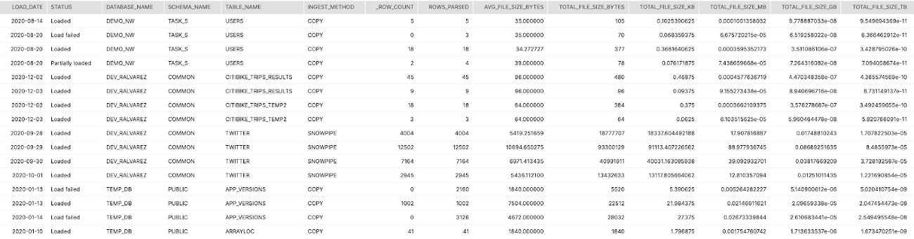
This query returns an aggregated daily summary of all loads for each table in Snowflake showing average file size, total rows, total volume and the ingest method (copy or snowpipe)

How to Interpret Results:

With this high-level information you can determine if file sizes are too small or too big for optimal ingest. If you can map the volume to credit consumption you can determine which tables are consuming more credits per TB loaded.

Primary Schema:

Account_Usage

SQL

SELECT 
  TO_DATE(LAST_LOAD_TIME) as LOAD_DATE
  ,STATUS
  ,TABLE_CATALOG_NAME as DATABASE_NAME
  ,TABLE_SCHEMA_NAME as SCHEMA_NAME
  ,TABLE_NAME
  ,CASE WHEN PIPE_NAME IS NULL THEN 'COPY' ELSE 'SNOWPIPE' END AS INGEST_METHOD
  ,SUM(ROW_COUNT) as ROW_COUNT
  ,SUM(ROW_PARSED) as ROWS_PARSED
  ,AVG(FILE_SIZE) as AVG_FILE_SIZE_BYTES
  ,SUM(FILE_SIZE) as TOTAL_FILE_SIZE_BYTES
  ,SUM(FILE_SIZE)/POWER(1024,1) as TOTAL_FILE_SIZE_KB
  ,SUM(FILE_SIZE)/POWER(1024,2) as TOTAL_FILE_SIZE_MB
  ,SUM(FILE_SIZE)/POWER(1024,3) as TOTAL_FILE_SIZE_GB
  ,SUM(FILE_SIZE)/POWER(1024,4) as TOTAL_FILE_SIZE_TB
FROM "SNOWFLAKE"."ACCOUNT_USAGE"."COPY_HISTORY"
GROUP BY 1,2,3,4,5,6
ORDER BY 3,4,5,1,2
;

Screenshot

alt-text-here

4. Scale Up vs. Out (Size vs. Multi-cluster) (T2)

Tier 2

Description:

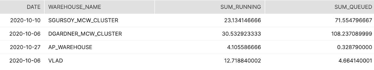
Two separate queries that list out the warehouses and times that could benefit from either a MCW setting OR scaling up to a larger size

How to Interpret Results:

Use this list to determine reconfiguration of a warehouse and the times or users that are causing contention on the warehouse

Primary Schema:

Account_Usage

SQL

--LIST OF WAREHOUSES AND DAYS WHERE MCW COULD HAVE HELPED
SELECT TO_DATE(START_TIME) as DATE
,WAREHOUSE_NAME
,SUM(AVG_RUNNING) AS SUM_RUNNING
,SUM(AVG_QUEUED_LOAD) AS SUM_QUEUED
FROM "SNOWFLAKE"."ACCOUNT_USAGE"."WAREHOUSE_LOAD_HISTORY"
WHERE TO_DATE(START_TIME) >= DATEADD(month,-1,CURRENT_TIMESTAMP())
GROUP BY 1,2
HAVING SUM(AVG_QUEUED_LOAD) >0
;

--LIST OF WAREHOUSES AND QUERIES WHERE A LARGER WAREHOUSE WOULD HAVE HELPED WITH REMOTE SPILLING
SELECT QUERY_ID
,USER_NAME
,WAREHOUSE_NAME
,WAREHOUSE_SIZE
,BYTES_SCANNED
,BYTES_SPILLED_TO_REMOTE_STORAGE
,BYTES_SPILLED_TO_REMOTE_STORAGE / BYTES_SCANNED AS SPILLING_READ_RATIO
FROM "SNOWFLAKE"."ACCOUNT_USAGE"."QUERY_HISTORY"
WHERE BYTES_SPILLED_TO_REMOTE_STORAGE > BYTES_SCANNED * 5  -- Each byte read was spilled 5x on average
ORDER BY SPILLING_READ_RATIO DESC
;

Screenshot

alt-text-here

5. Warehouse Cache Usage (T3)

Tier 3

Description:

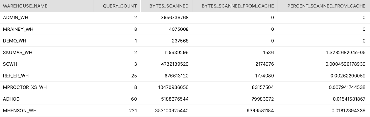
Aggregate across all queries broken out by warehouses showing the percentage of data scanned from the warehouse cache.

How to Interpret Results:

Look for warehouses that are used from querying/reporting and have a low percentage. This indicates that the warehouse is suspending too quickly

Primary Schema:

Account_Usage

SQL

SELECT WAREHOUSE_NAME
,COUNT(*) AS QUERY_COUNT
,SUM(BYTES_SCANNED) AS BYTES_SCANNED
,SUM(BYTES_SCANNED*PERCENTAGE_SCANNED_FROM_CACHE) AS BYTES_SCANNED_FROM_CACHE
,SUM(BYTES_SCANNED*PERCENTAGE_SCANNED_FROM_CACHE) / SUM(BYTES_SCANNED) AS PERCENT_SCANNED_FROM_CACHE
FROM "SNOWFLAKE"."ACCOUNT_USAGE"."QUERY_HISTORY"
WHERE START_TIME >= dateadd(month,-1,current_timestamp())
AND BYTES_SCANNED > 0
GROUP BY 1
ORDER BY 5
;

Screenshot

alt-text-here

6. Heavy Scanners (T3)

Tier 3

Description:

Ordered list of users that run queries that scan a lot of data.

How to Interpret Results:

This is a potential opportunity to train the user or enable clustering.

Primary Schema:

Account_Usage

SQL

select 
  User_name
, warehouse_name
, avg(case when partitions_total > 0 then partitions_scanned / partitions_total else 0 end) avg_pct_scanned
from   snowflake.account_usage.query_history
where  start_time::date > dateadd('days', -45, current_date)
group by 1, 2
order by 3 desc
;

7. Full Table Scans by User (T3)

Tier 3

Description:

These queries are the list of users that run the most queries with near full table scans and then the list of the queries themselves.

How to Interpret Results:

This is a potential opportunity to train the user or enable clustering.

Primary Schema:

Account_Usage

SQL

--who are the users with the most (near) full table scans
SELECT USER_NAME
,COUNT(*) as COUNT_OF_QUERIES
FROM "SNOWFLAKE"."ACCOUNT_USAGE"."QUERY_HISTORY"
WHERE START_TIME >= dateadd(month,-1,current_timestamp())
AND PARTITIONS_SCANNED > (PARTITIONS_TOTAL*0.95)
AND QUERY_TYPE NOT LIKE 'CREATE%'
group by 1
order by 2 desc;

-- This gives all queries in the last month with nearly a full table scan :) > 95%, ordered by the worst offending
SELECT * 
FROM "SNOWFLAKE"."ACCOUNT_USAGE"."QUERY_HISTORY"
WHERE START_TIME >= dateadd(month,-1,current_timestamp())
AND PARTITIONS_SCANNED > (PARTITIONS_TOTAL*0.95)
AND QUERY_TYPE NOT LIKE 'CREATE%'
ORDER BY PARTITIONS_SCANNED DESC
LIMIT 50  -- Configurable threshold that defines "TOP N=50"
;

8. Top 10 Spillers Remote (T3)

Tier 3

Description:

Identifies the top 10 worst offending queries in terms of bytes spilled to remote storage.

How to Interpret Results:

These queries should most likely be run on larger warehouses that have more local storage and memory.

Primary Schema:

Account_Usage

SQL

select query_id, substr(query_text, 1, 50) partial_query_text, user_name, warehouse_name, warehouse_size, 
       BYTES_SPILLED_TO_REMOTE_STORAGE, start_time, end_time, total_elapsed_time/1000 total_elapsed_time
from   snowflake.account_usage.query_history
where  BYTES_SPILLED_TO_REMOTE_STORAGE > 0
and start_time::date > dateadd('days', -45, current_date)
order  by BYTES_SPILLED_TO_REMOTE_STORAGE desc
limit 10
;

9. AutoClustering History & 7-Day Average (T3)

Tier 3

Description:

Average daily credits consumed by Auto-Clustering grouped by week over the last year.

How to Interpret Results:

Look for anomalies in the daily average over the course of the year. Opportunity to investigate the spikes or changes in consumption.

Primary Schema:

Account_Usage

SQL

WITH CREDITS_BY_DAY AS (
SELECT TO_DATE(START_TIME) as DATE
,SUM(CREDITS_USED) as CREDITS_USED


FROM "SNOWFLAKE"."ACCOUNT_USAGE"."AUTOMATIC_CLUSTERING_HISTORY"

WHERE START_TIME >= dateadd(year,-1,current_timestamp()) 
GROUP BY 1
ORDER BY 2 DESC 
  )
  
SELECT DATE_TRUNC('week',DATE)
,AVG(CREDITS_USED) as AVG_DAILY_CREDITS
FROM CREDITS_BY_DAY
GROUP BY 1
ORDER BY 1
;

10. Materialized Views History & 7-Day Average (T3)

Tier 3

Description:

Average daily credits consumed by Materialized Views grouped by week over the last year.

How to Interpret Results:

Look for anomalies in the daily average over the course of the year. Opportunity to investigate the spikes or changes in consumption.

Primary Schema:

Account_Usage

SQL

WITH CREDITS_BY_DAY AS (
SELECT TO_DATE(START_TIME) as DATE
,SUM(CREDITS_USED) as CREDITS_USED


FROM "SNOWFLAKE"."ACCOUNT_USAGE"."MATERIALIZED_VIEW_REFRESH_HISTORY"

WHERE START_TIME >= dateadd(year,-1,current_timestamp()) 
GROUP BY 1
ORDER BY 2 DESC 
  )
  
SELECT DATE_TRUNC('week',DATE)
,AVG(CREDITS_USED) as AVG_DAILY_CREDITS
FROM CREDITS_BY_DAY
GROUP BY 1
ORDER BY 1
;

11. Search Optimization History & 7-Day Average (T3)

Tier 3

Description:

Average daily credits consumed by Search Optimization grouped by week over the last year.

How to Interpret Results:

Look for anomalies in the daily average over the course of the year. Opportunity to investigate the spikes or changes in consumption.

Primary Schema:

Account_Usage

SQL

WITH CREDITS_BY_DAY AS (
SELECT TO_DATE(START_TIME) as DATE
,SUM(CREDITS_USED) as CREDITS_USED


FROM "SNOWFLAKE"."ACCOUNT_USAGE"."SEARCH_OPTIMIZATION_HISTORY"

WHERE START_TIME >= dateadd(year,-1,current_timestamp()) 
GROUP BY 1
ORDER BY 2 DESC 
  )
  
SELECT DATE_TRUNC('week',DATE)
,AVG(CREDITS_USED) as AVG_DAILY_CREDITS
FROM CREDITS_BY_DAY
GROUP BY 1
ORDER BY 1
;

12. Snowpipe History & 7-Day Average (T3)

Tier 3

Description:

Average daily credits consumed by Snowpipe grouped by week over the last year.

How to Interpret Results:

Look for anomalies in the daily average over the course of the year. Opportunity to investigate the spikes or changes in consumption.

Primary Schema:

Account_Usage

SQL

WITH CREDITS_BY_DAY AS (
SELECT TO_DATE(START_TIME) as DATE
,SUM(CREDITS_USED) as CREDITS_USED


FROM "SNOWFLAKE"."ACCOUNT_USAGE"."PIPE_USAGE_HISTORY"

WHERE START_TIME >= dateadd(year,-1,current_timestamp()) 
GROUP BY 1
ORDER BY 2 DESC 
  )
  
SELECT DATE_TRUNC('week',DATE)
,AVG(CREDITS_USED) as AVG_DAILY_CREDITS
FROM CREDITS_BY_DAY
GROUP BY 1
ORDER BY 1
;

13. Replication History & 7-Day Average (T3)

Tier 3

Description:

Average daily credits consumed by Replication grouped by week over the last year.

How to Interpret Results:

Look for anomalies in the daily average over the course of the year. Opportunity to investigate the spikes or changes in consumption.

Primary Schema:

Account_Usage

SQL

WITH CREDITS_BY_DAY AS (
SELECT TO_DATE(START_TIME) as DATE
,SUM(CREDITS_USED) as CREDITS_USED


FROM "SNOWFLAKE"."ACCOUNT_USAGE"."REPLICATION_USAGE_HISTORY"

WHERE START_TIME >= dateadd(year,-1,current_timestamp()) 
GROUP BY 1
ORDER BY 2 DESC 
  )
  
SELECT DATE_TRUNC('week',DATE)
,AVG(CREDITS_USED) as AVG_DAILY_CREDITS
FROM CREDITS_BY_DAY
GROUP BY 1
ORDER BY 1
;

Back